Examples

Here we provide a few examples for using package.

Find coexisting phases once

Since we only need to find the coexisting phases once, we assign values to the \(\chi_{ij}\) matrix and the average volume fractions \(\bar{\phi}_i\) , and call the wrapper function find_coexisting_phases() directly. Here we consider a symmetric two-component system, with \(\chi=4\):

import flory

chis = [[0, 4.0], [4.0, 0]]
phi_means = [0.5, 0.5]

phases = flory.find_coexisting_phases(2, chis, phi_means)

with open(__file__ + ".out", "w") as f:
    print("Volumes:", phases.volumes, file=f)
    print("Compositions:", phases.fractions, file=f)

We obtain two symmetric phases:

Volumes: [0.5 0.5]
Compositions: [[0.97875201 0.02124799]
 [0.02124799 0.97875201]]

By adding a sizes parameter, we can also investigate the coexisting phases where the components have different molecule sizes:

import flory

chis = [[0, 4.0], [4.0, 0]]
phi_means = [0.5, 0.5]
sizes = [1.0, 2.0]

phases = flory.find_coexisting_phases(2, chis, phi_means, sizes=sizes)

with open(__file__ + ".out", "w") as f:
    print("Volumes:", phases.volumes, file=f)
    print("Compositions:", phases.fractions, file=f)

which gives two asymmetric phases:

Volumes: [0.49421383 0.50578617]
Compositions: [[9.99096418e-01 9.02812053e-04]
 [1.23228537e-02 9.87677899e-01]]

Extension to more components is straight forward:

import flory

chis = [[3.27, -0.34, 0], [-0.34, -3.96, 0], [0, 0, 0]]
phi_means = [0.16, 0.55, 0.29]
sizes = [2.0, 2.0, 1.0]

phases = flory.find_coexisting_phases(3, chis, phi_means, sizes=sizes)

with open(__file__ + ".out", "w") as f:
    print("Volumes:", phases.volumes, file=f)
    print("Compositions:", phases.fractions, file=f)

which gives two phases:

Volumes: [0.63347743 0.36652257]
Compositions: [[0.07578503 0.81378509 0.11042987]
 [0.30555252 0.09408838 0.60035913]]

Construct a 2D phase diagram

When constructing a phase diagram, we usually need to find coexisting phases for multiple instances. To avoid the creation and the destruction of the internal data each time, we provide the class API CoexistingPhasesFinder. Using the class API usually involves three steps: creation of the finder instance, setting the system parameters and finding the coexisting states. When the system sizes such as number of components \(N_\mathrm{C}\) and the number of compartments \(N_\mathrm{M}\) do not change, the finder can be reused. 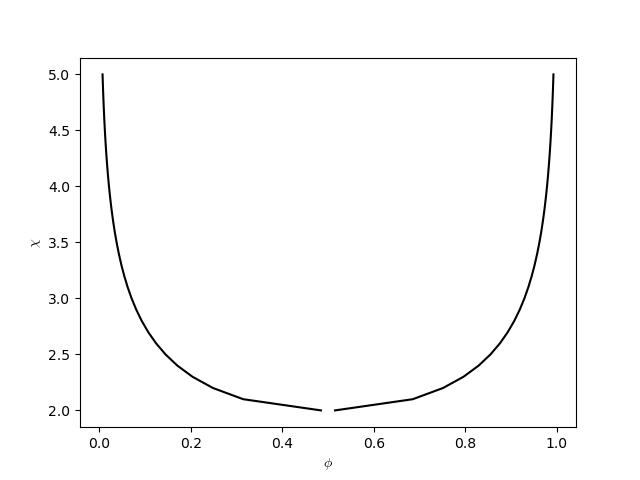Here we provide a simple example for generating a \((\phi, \chi)\) phase diagram for a simple binary mixture:

import matplotlib.pyplot as plt
import numpy as np

import flory

chi_start = 5.0
chi_end = 1.0

num_comp = 2
chis = [[0.0, 0.0], [0.0, 0.0]]
phi_means = [0.5, 0.5]

free_energy = flory.FloryHuggins(num_comp, chis)
interaction = free_energy.interaction
entropy = free_energy.entropy
ensemble = flory.CanonicalEnsemble(num_comp, phi_means)
finder = flory.CoexistingPhasesFinder(
    interaction,
    entropy,
    ensemble,
    progress=False,
)


line_chi = []
line_l = []
line_h = []
for chi in np.arange(chi_start, chi_end, -0.1):  # scan chi from high value to low value
    interaction.chis = np.array([[0, chi], [chi, 0]])  # set chi matrix of the finder
    finder.set_interaction(interaction)
    phases = finder.run().get_clusters()  # get coexisting phases
    if phases.fractions.shape[0] == 1:  # stop scanning if no phase separation
        break
    phi_h = phases.fractions[
        0, 0
    ]  # extract the volume fraction of component 0 in phase 0
    phi_l = phases.fractions[
        1, 0
    ]  # extract the volume fraction of component 0 in phase 1
    line_chi.append(chi)
    line_l.append(phi_l)
    line_h.append(phi_h)

plt.plot(line_l, line_chi, c="black")
plt.plot(line_h, line_chi, c="black")
plt.xlabel("$\\phi$")
plt.ylabel("$\\chi$")
plt.savefig(__file__ + ".jpg")

We obtain the phase diagram

Check finite size effect

The minimization process in our algorithm DO NOT guarantee that the equilibrium state is always found. Due to the multistability of the multicomponent mixture, tt is possible that the algorithm find a local minimum. For example, the true equilibrium state can be a 4-phase coexisting state, while the algorithm may find a metastable 3-phase coexisting state. This issue can be resolved by launching more compartments than phases. Obviously, the maximum number of phases can be found is always not larger than the number of the compartments. By launching more compartments, it makes the algorithm much more likely to find the correct coexisting states. Here we refer to this as the finite size effect, see an example of \(N_\mathrm{C}=8\) below:

import matplotlib.pyplot as plt
import numpy as np

import flory

N_comp = 8

# create a random chi matrix
chi_mean = 0
chi_std = 8
rng = np.random.default_rng(2333)
chis = rng.normal(chi_mean, chi_std, (N_comp, N_comp))
chis = 0.5 * (chis + chis.T)
chis *= 1.0 - np.identity(N_comp)

phi_means = np.full(N_comp, 1.0 / N_comp)  # set a symmetric composition

line_N_compartment = []
line_N_phase = []
for N_compartment in range(4, 16, 2):  # use different compartment number
    phases = flory.find_coexisting_phases(
        N_comp, chis, phi_means, num_part=N_compartment, progress=True
    )
    line_N_compartment.append(N_compartment)
    line_N_phase.append(phases.volumes.shape[0])

plt.plot(line_N_compartment, line_N_phase, c="black")
plt.xlabel("number of compartments")
plt.ylabel("number of phases")
plt.savefig(__file__ + ".jpg")

We obtain

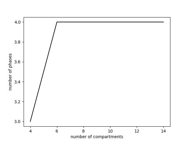
showing that \(N_\mathrm{M}=4\) underestimates the number of phases in the final coexisting state, while larger \(N_\mathrm{M}\) values give the correct result.

Construct a ternary phase diagram

Here we provide a simple example for generating a \((\phi_B, \phi_A)\) phase diagram for a simple ternary mixture with fixed interaction matrix. The example first finds a point in the phase diagram that leads to three-phase coexistence, which is a triangle in the phase diagram. Then starting from each edge of the triangle, we follow the direction to the unknown region in the phase diagram to complete all two-phase coexistence regions.

import matplotlib.pyplot as plt
import numpy as np

import flory

num_comp = 3
chis = [[0.0, 2.4, 3.2], [2.4, 0.0, 2.8], [3.2, 2.8, 0.0]]
# we guess this point is a three-phase coexistence point
phi_means = [0.33, 0.33, 0.34]

free_energy = flory.FloryHuggins(num_comp, chis)
interaction = free_energy.interaction
entropy = free_energy.entropy
ensemble = flory.CanonicalEnsemble(num_comp, phi_means)
options = {
    "num_part": 8,
    "progress": False,
    "max_steps": 10000000,  # disable progress bar, allow more steps
}
finder = flory.CoexistingPhasesFinder(interaction, entropy, ensemble, **options)

# determine the three phase coexistence
phases = finder.run().get_clusters()
assert phases.volumes.shape[0] == 3
p3_phis = phases.fractions
p3_center = np.mean(p3_phis, axis=0)
p3_edges = [p3_phis[[1, 2]], p3_phis[[0, 2]], p3_phis[[0, 1]]]


# function that scan the 2-phase coexistence until the boundary is reached
def find_p2_boundaries(
    init_tie: np.ndarray,
    start_point: np.ndarray,
    finder: flory.CoexistingPhasesFinder,
    scan_step: float = 0.02,
    scan_step_min: float = 0.000001,
):
    internal_finder = flory.CoexistingPhasesFinder(
        interaction, entropy, ensemble, **options
    )

    internal_finder.reinitialize_from_omegas(
        finder.omegas.copy()
    )  # use previous internal fields to accelerate

    previous = start_point
    current_tie = init_tie
    step = scan_step

    ties = [init_tie]
    while True:
        tie_center = current_tie.mean(axis=0)
        tie_dir = current_tie[1] - current_tie[0]
        tie_dir = tie_dir / np.linalg.norm(tie_dir)
        next_dir = tie_center - previous
        next_dir = next_dir - np.dot(next_dir, tie_dir) * tie_dir
        next_dir = next_dir / np.linalg.norm(next_dir)
        next_phis = tie_center + step * next_dir

        ensemble.phi_means = np.array(next_phis)
        internal_finder.set_ensemble(ensemble)
        backup_omegas = internal_finder.omegas.copy()
        phases = internal_finder.run().get_clusters()

        if phases.volumes.shape[0] == 2 and np.all(phases.fractions > 0):
            ties.append(phases.fractions)
            previous = tie_center
            current_tie = phases.fractions
        else:
            internal_finder.reinitialize_from_omegas(backup_omegas)
            if step > scan_step_min:
                step /= 2
            else:
                break

    return np.array(ties)


p2_ties = [find_p2_boundaries(edge, p3_center, finder) for edge in p3_edges]

# plot the allowed region
plt.plot([0, 1, 0, 0], [1, 0, 0, 1], c="black")

for ties in p2_ties:
    # plot the phase boundaries
    plt.plot(ties[:, 0, 0], ties[:, 0, 1], c="brown")
    plt.plot(ties[:, 1, 0], ties[:, 1, 1], c="brown")
    for tie in ties:
        # plot the tie lines
        plt.plot(tie[:, 0], tie[:, 1], c="gray")

# plot the 3-phase region
plt.plot(p3_phis[[0, 1, 2, 0], 0], p3_phis[[0, 1, 2, 0], 1], c="blue")

plt.xlabel("$\\phi_A$")
plt.ylabel("$\\phi_B$")
plt.savefig(__file__ + ".jpg")

We obtain the phase diagram

Using constraints

In many systems such as mixtures containing ions or chemical reactions, there are additional constraints. flory provides convenient ways to consider these constrains. For example, in a system with 5 components, with first four components are charged, flory can find the coexisting phases that each phase is charge neutral, by applying a LinearLocalConstraint:

import numpy as np

import flory

num_comp = 5
chis = np.zeros((num_comp, num_comp))
chis[0][1] = -7.0
chis[1][0] = -7.0
phi_means = [0.10, 0.10, 0.09, 0.09, 0]
phi_means[4] = 1.0 - np.sum(phi_means)
sizes = [10.0, 10.0, 1.0, 1.0, 1.0]

Cs = [0.9, -0.9, -1, 1, 0]
Ts = 0

fh = flory.FloryHuggins(num_comp, chis, sizes=sizes)
ensemble = flory.CanonicalEnsemble(num_comp, phi_means)
constraint = flory.LinearLocalConstraint(num_comp, Cs, Ts)

finder = flory.CoexistingPhasesFinder(
    fh.interaction,
    fh.entropy,
    ensemble,
    [constraint],
    max_steps=1000000,
    progress=True,
)
phases = finder.run().get_clusters()

with open(__file__ + ".out", "w") as f:
    print("Volumes:", phases.volumes, file=f)
    print("Compositions:", phases.fractions, file=f)

Using different ensemble

When considering an open system, the volume fractions are no longer conserved. Instead, the system will keep fixed chemical potentials. flory can handle this by switching from CanonicalEnsemble to GrandCanonicalEnsemble:

import numpy as np

import flory

num_comp = 3
chis = (1 - np.identity(num_comp)) * 5

mus = [-1, 0.0, 0.1]

Cs = [[1, 1, 0]]
Ts = [0.4]

fh = flory.FloryHuggins(num_comp, chis)
ensemble = flory.GrandCanonicalEnsemble.from_chemical_potential(num_comp, mus)
constraint = flory.LinearGlobalConstraint(num_comp, Cs, Ts)

finder = flory.CoexistingPhasesFinder(
    fh.interaction,
    fh.entropy,
    ensemble,
    constraint,
    random_std=1.0,  # use less aggressive randomness to avoid rapid dying of compartments
    progress=True,
    tolerance=1e-12,
)
phases = finder.run().get_clusters()

with open(__file__ + ".out", "w") as f:
    print("Volumes:", phases.volumes, file=f)
    print("Compositions:", phases.fractions, file=f)

Using different interaction&entropy

In a mixture with polydispersity, several components may share the same interaction property but only differs in size. flory allows to handle this case sufficiently by using different interaction and entropy:

import numpy as np

import flory

num_feat = 2
chis_feat = [[0, 4.0], [4.0, 0]]
phi_means = [0.2, 0.3, 0.2, 0.3]
sizes = [1, 2, 1, 2]
num_comp_per_feat = [2, 2]
num_comp = np.sum(num_comp_per_feat)

interaction = flory.FloryHugginsBlockInteraction(num_feat, chis_feat, num_comp_per_feat)
entropy = flory.IdealGasPolydispersedEntropy(num_feat, sizes, num_comp_per_feat)
ensemble = flory.CanonicalEnsemble(num_comp, phi_means)
finder = flory.CoexistingPhasesFinder(interaction, entropy, ensemble)

phases = finder.run().get_clusters()

with open(__file__ + ".out", "w") as f:
    print("Volumes:", phases.volumes, file=f)
    print("Compositions:", phases.fractions, file=f)